In this tutorial we'll consider five functions every Blender user should know: Sine, Cosine, Logarithm, Power and Modulo. If you've ever studied digital signals processing or sound synthesis, you will recognise these functions as old friends.
Looking at the Math node in Blender, we see a number of other operators as well. Most of them, like Multiply, Subtract, Add, etc. are easy to understand, while Arcsine and its siblings are of limited use, as modulating functions mostly.
The Sine is probably the most useful of them all. As
explained on Wikipedia, Sine is a trigonometric function, closely related to the circle. The beauty of Sine is that with growing input such as the X axis or the timeline, the Sine outputs values between -1 and 1 in the shape of an oscillating wave. The Cosine is practically the same, the only difference being the 1/4 offset between the two: Sine begins at 0 but Cosine begins at 1.
Because of their similarity, the Sine is usually used, except when the phase of Cosine is more desirable.
While the output range of -1 to 1 is very neat and helpful in calculations, the frequency of the cycles is less neat: one cycle completes every 6.2832 units of input, that is 2*Pi. In graphics use, the number seems rather arbitrary - how can we "normalize" the cycles down to 1 cycle per 1 unit of input? Easy, we multiply the input by 6.2832. In doing so, we've achieved a reduction of the frequency, an operation we'll perform often.
It will also help us to convert the -1 to 1 output to a more relevant 0-1 range, given that colour values can be expressed in this range. Easily done: we add 1 to the output to bring it to the 0-2 range, and divide by 2 to obtain the range of 0-1. The midpoint of the range is now 0.5, not 0.
We're doing well so far, but when we look at more of the waves over a longer span of input values, we see how uniform they are. In most cases, we'll want to vary - or modulate - the output. Let's say we want to vary the height of the waveforms, so that they don't always reach the extremes of the range. What sort of calculation would achieve this?
The clue is in the output range of our Sine itself: if maximum values range between 0 and 1, and we want to variably reduce the output within this range, then it follows that the effect will be achieved if we multiply the output with values between 0 and 1. Are you getting it? We can modulate the output of a Sine by multiplying with the output of another Sine! For a nice effect, the modulating Sine should be of longer wavelength.
You can see we've constructed a ten times longer waveform for the modulating Sine, by multiplying the input with 0.1.
If we now multiply the output of the original Sine with the modulating Sine, we see the effect. The waveforms are no longer of a uniform, maximum height, but vary according to the shape of the modulating wave.
Yet, over a longer span of X values, the uniformity of the output is once again apparent. Can we modulate it some more?
Of course we can, we multiply the output by yet another Sine. Notice in the example image that I no longer multiply the input by 6.2832, as that is by now quite redundant. We're not so concerned at this moment that the wavelength be 1 cycle per 1 X unit. Notice also that I'm multiplying the modulating Sine inputs by 0.05 and 0.04 to obtain a nice look for the variation.
We could carry on this process of modulating the amplitude of the waveforms, but let's try something new: can we modulate the frequency? Let's say we don't want it to be perfectly uniform. What is the calculation for this? We've already seen that if left unchanged, the frequency is 1 cycle per 6.2832 X units. If we want this to vary a little, just enough to overcome the uniformity, then the frequency should vary between 5 and 7 X units or thereabouts. Are you getting it, again?
You guessed right, if we add the output of a modulating Sine (that hasn't been normalized) to the input of the original Sine, we'll have a frequency range varying between 5.2832 and 7.2832 X units. Further still, if we multiply the input of the modulating Sine by 0.5, then the variation will occur over double the wavelength of the original Sine. Now we've obtained a fairly natural-looking waveform that could be used to represent a soundwave in a graphic.
Before we move on to a practical application of what we have learned, let's look at a couple of the other functions. Starting with Modulo - what does it do? As
Wikipedia explains, modulo gives us the remainder of a division. That doesn't sound very promising, does it? We're not all that interested in remainders of a division usually.
The penny drops, however, when we realize that with any given divisor, on growing input, the remainders will keep rising until the input equals the divisor, then the remainder drops to 0, and the cycle begins again. Modulo is rather similar to the Sine then, except its output is between 0 and the divisor, and the frequency is equal in length to the divisor too. The linear rise and sudden drop to 0 give the wave its sawtooth look.
Represented graphically, the Modulo is good for generating tree rings in wood. For more details about creating a wood material with Modulo, see Bartek Skorupa's excellent #BCon14 presentation
Manipulate texture coordinates like a boss.
All of the modulating principles already discussed in relation to the Sine also apply to the Modulo. ("Modulo" and "modulating" sound similar but are two different things.)
Next,
Logarithm; one of the exponential functions. In its inverse form, it is useful as a damping modulator. In the example graphic, the curve is inverted by dividing the input into 1, and tempered by adding 2 to the value of X. The larger this addition, the flatter the curve would be. Finally, the output is normalized to the output range of 0-1.
If we multiply a Sine curve by the Logarithm function created above (named
logY here), we obtain the damping of the Sine. This brings us neatly to
Power, the fifth function in our set. Power is exponentiation, "raising to the power of", squaring or cubing that we learnt about in high school. In our case, we raise our Sine to the power of 0.3, and that changes the Sine curve to appear as hills in the "boing boing" curve of a bouncing ball.
That's the beauty of Power at fractional settings below 1 - it will have greater positive effect on numbers closer to 0 than those close to 1, hence the sharp 0 touchdowns we see in the result.
Enough of the explanations, let's now see if we can play with these functions in Blender directly. It would be useful if we could construct them in a Cycles material, immediate preview of the result in the Rendered viewport allowing us to play with the settings at will.
To accomplish this feat, we create a Plane of 1 x 1 dimensions. We'll be using Object coordinates for its material mapping. The origin in this mapping being the origin of the object, it helps if we move the origin to the lower left vertex, so the material can "fill" the Plane from there.
For a perspective-free view of the Plane, we switch to the Top orthographic view, press Ctl-Alt-0 on Numpad to Align Active Camera to View, press . on the Numpad to position the Plane squarely in the view, and change the Camera Lens setting to Orthographic and Scale of 1 for a perfect, tight capture of the Plane.
 |
| Click to enlarge |
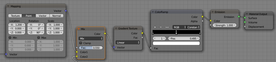
Our objective is to create a horizontal line across the Plane, that we could then shape into a curve with our math. To create the line, we assign a new Emission material to the Plane, and feed the output of a Linear Gradient Texture into a ColorRamp. We convert the gradient into a line by using a very narrow Constant stretch of white in the middle of the ColorRamp range (0.495-0.501). The Mix node is there to mix the curve generating node outputs to the Vector, and the mapping node positions the texture correctly on the Plane.
 |
| Click to enlarge |
Having set up the flat white line across the Plane, we now add the math nodes to shape it into our boing boing curve. As you can see in the screen capture, our math is practically the same as it was in the examples above. We separate the Object texture coordinate vector with a Separate RGB node (RGB and Vectors are really the same thing) and work on the R, or X, component. The upper row, containing the Sine, shapes the undamped boing boing curve, while the lower row containing the Logarithm, provides the damping.
The two highlighted nodes on the very left of the node tree are new: they provide damping of the frequency. Without it, each hill of the curve would have the same X length, and that's not natural. The X length of the hills should decrease as the hills become smaller.
 |
| Click to enlarge |
We've been very good so far, now it's time to go crazy. We should be able to use our setup -
sans the damping Logarithm - to create linear patterns that we could use in wallpapers and other ornamentation. The key is to experiment - change everything and anything to your heart's content.
Given that we are now "masters of the curve", could we do more? How about creating a boing boing spline curve that we could use to animate a ball? We could do that and here's the script for it, but there are problems with this approach. You should treat the script as proof of concept only, it isn't practically useful. Copy and paste the script into the Text Editor, press Run Script, then in 3D View, press Spacebar and type "Boing Curve".
import bpy
import math

def MyFunction(context):
 scene = context.scene
 cursor = scene.cursor_location

 curve = bpy.data.scenes.data.curves.new(name="BoingCurve", type='CURVE')

 obj = bpy.data.scenes.data.objects.new(name="BoingCurve", object_data=curve)
 scene.objects.link(obj)
 obj.location = cursor

 bpy.context.scene.objects.active = obj
 bpy.context.scene.objects.active.select = True

 bpy.ops.object.editmode_toggle()
 for x in range(1,500): # prevent division of 0
  x = x/500
  dampLog = abs(math.log1p(1/(x+0.2))*1)-0.6
  z = math.pow((math.sin(x*40)+1)*0.5,0.3)*dampLog
  bpy.ops.curve.vertex_add(location=(x, 0.0, z))
  bpy.ops.curve.handle_type_set(type='VECTOR')
 bpy.ops.object.editmode_toggle()

class MyOperator(bpy.types.Operator):
 '''Create a Boing Curve'''
 bl_idname = "object.boing_curve"
 bl_label = "Boing Curve"
 bl_options = {"REGISTER", "UNDO"}

 def execute(self, context):
  MyFunction(context)
  return {'FINISHED'}

def register():
 bpy.utils.register_module(__name__)


def unregister():
 bpy.utils.unregister_module(__name__)

if __name__ == '__main__':
 register()

Here you see a spline curve created by the script. Because the spline is constructed from vertices, its resolution is finite, which means that the 0 value is easily missed and the curve won't "touch down" to 0. An additional calculation could fix that, but there isn't much point, as this curve is less useful for animation than you might hope. If you animate a ball along it, the speed will not appear natural. There are easier ways of obtaining a realistic bouncing ball curve, namely the physics system in Blender.
A better bet is to return to our earlier example of a realistic sound wave. Here's the script - run it from the Text Editor as before, and in 3D View search for "Sound Curve".
import bpy
import math

def MyFunction(context):
 scene = context.scene
 cursor = scene.cursor_location

 curve = bpy.data.scenes.data.curves.new(name="SoundCurve", type='CURVE')

 obj = bpy.data.scenes.data.objects.new(name="SoundCurve", object_data=curve)
 scene.objects.link(obj)
 obj.location = cursor

 bpy.context.scene.objects.active = obj
 bpy.context.scene.objects.active.select = True

 bpy.ops.object.editmode_toggle()
 for x in range(1,500): # prevent division of 0
  x = x/500
  y = (math.sin((x+(math.sin(x*62)))*125)*math.sin(x*7)*math.sin(x*9)*math.sin(x*12)+1)*0.5
  bpy.ops.curve.vertex_add(location=(x, y, 0.0))
  bpy.ops.curve.handle_type_set(type='VECTOR')
 bpy.ops.object.editmode_toggle()

class MyOperator(bpy.types.Operator):
 '''Create a Sound Curve'''
 bl_idname = "object.sound_curve"
 bl_label = "Sound Curve"
 bl_options = {"REGISTER", "UNDO"}

 def execute(self, context):
  MyFunction(context)
  return {'FINISHED'}

def register():
 bpy.utils.register_module(__name__)


def unregister():
 bpy.utils.unregister_module(__name__)

if __name__ == '__main__':
 register()

With the curve in place, you could add a bevel to it, apply an Emission shader, and you'll soon have a soundwave background. You could animate a pulsating ball to travel along it at great speed... With your newly gained knowledge, you should be able to create new curves without too much difficulty. Play with the math nodes to obtain the shape you want, then transfer the math into the script.
To wrap this up, I'll leave you with a couple more examples of these functions in use. Don't be afraid to experiment and you'll soon be using these five essential functions to great effect in your own work.
 |
| Click to enlarge |
 |
| Click to enlarge |


very very informative article thankyou,
ReplyDeleteHowever i would like to suggest if at all possible,
How's about giving the readers a pdf to download, at least then we could look offline as much as on,
Plus it also gives us a extra document to add to our understanding & learning blender folders again cheers for the very useful information very much appreciated,
Thankyou